ERDDAP is a great and increasingly common tool for accessing different time series data. On the surface, it allows users to make requests and basic plots using the webpage. While some of the interface may look complicated, there isn't much to be afraid of. Since all of the processing and requests are done on the server side, you can always start over or try again if things aren't working as they should be.
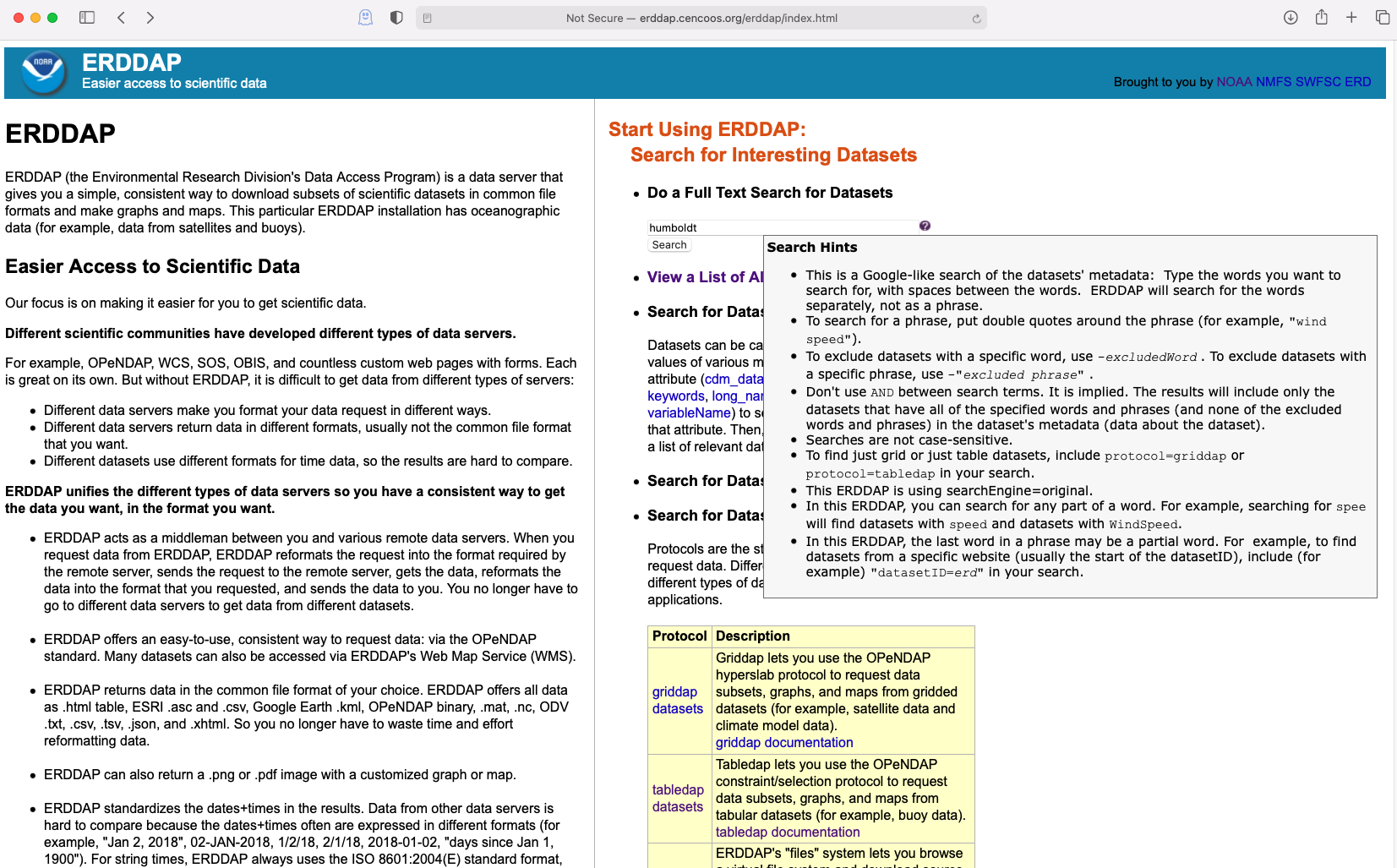
Try navigating to the CeNCOOS ERDDAP page: erddap.cencoos.org
and searching for the station. The search is fairly elastic and will look through both the dataset title and id, as well as metadata which can include keywords.
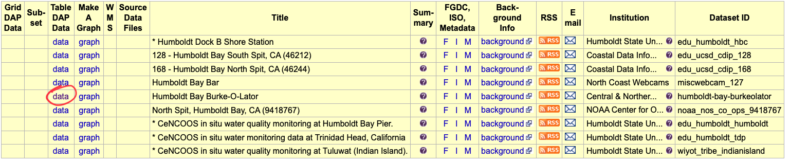
For example try searching for Humboldt
or burkeolator
We just want to get to the data, so select the data tab for the Humboldt Burke-o-lator dataset
Now we want to make use the Optional Constraint field to query only data where the Salinity QC is flagged as 1 (Pass) and not 3 (Suspect) nor 4 (Fail).
First, make sure to put a check mark for the variables that you are interested in and uncheck the ones we don't want. This will help keep the file size down and ensure that the request that we are going to make is fast.
Make sure to ajust the time slider to get the length of time that is desired.
Then, next to the sea_water_practical_salinity_qc_agg select the equal
option from the dropdown menu and insert a value of 1
into Optional Contraint #1
field.
Now select the type of output that you want the data to be in, this is where ERDDAP really starts to show its strenght. ERDDAP can create almost any type of file that you want and will do it all on the backend, so you don't have to do anything!
Let's first select the .htmlTable
option to first view the data and make sure everything is working. The results should look like this.
Since this looks good, lets go back and select a .csv
to download. And hit the Submit
button to make the request to download the data.
One super useful thing, is that you don't need to actually download the file onto you machine if you are going to run an anlysis in python
or R
. Instead you can copy the request URL and open the file directly into memory.
Instead of clicking Submit, click the Just generate the URL
button.
This will give you a string that looks something like:
http://erddap.cencoos.org/erddap/tabledap/humboldt-bay-burkeolator.csv?time%2Comega_aragonite%2Csea_water_practical_salinity%2Csea_water_practical_salinity_qc_agg%2Csea_water_temperature%2Csea_water_temperature_qc_agg%2Csea_water_ph_reported_on_total_scale%2Csea_water_ph_reported_on_total_scale_qc_agg&time%3E=2021-06-16
Here is an example of how to access the data, run a low-pass filter, and plot the data, all with having to download anything!
import matplotlib.pyplot as plt
import pandas as pd
url = "http://erddap.cencoos.org/erddap/tabledap/humboldt-bay-burkeolator.csv?time%2Comega_aragonite%2Csea_water_practical_salinity%2Csea_water_practical_salinity_qc_agg%2Csea_water_temperature%2Csea_water_temperature_qc_agg%2Csea_water_ph_reported_on_total_scale%2Csea_water_ph_reported_on_total_scale_qc_agg&time%3E=2021-06-16"
df = pd.read_csv(url, skiprows=[1], infer_datetime_format=True, parse_dates=['time'], index_col='time')
df['sea_water_temperature'].plot(label='Raw')
# Create a 40 hour rolling low-pass filter
df['sea_water_temperature'].dropna().rolling(window=240*40,win_type='hamming').mean().plot(label='Filter')
plt.title("Humoblt BoL \n Sea Water Temperature - 40 Hour low-pass filter")
plt.ylabel('Temperature [C]')
plt.legend()
Text(0, 0.5, 'Temperature [C]')